Understanding Database IOPS – Part 1

Introduction:

Cloud has greatly simplified the process to deploy and manage databases. With RDS like offering most of the database maintenance activities like upgrades/backups/etc. are automated. That said, cloud introduces another challenge for end-user : How to select cost optimal configuration and still continue to achieve the needed throughput ?

Given database is IO intensive application one key-factor in this optimization is IOPS. This article will help explore cost effectiveness based on IOPS comparing different options available for managing DB in cloud.

What is IOPS?

Simple definition is Input/Output Operation per second. Databases are IO intensive they continuously modify data-pages, metadata, flushed undo/redo logs, persist tracking logs (audit/slow log), etc… Given this aspect of DB , it is important to wisely select IOPS. Also, limiting IOPS (to default) may cause database to hit threshold and considerably reduce performance. Over provisioning of IOPS will result in growing cost for managing an instance.

EBS Vs Instance store:

EC2 instances support two types for block-level storage

Elastic Block Store (EBS)
Instance Store (Ephemeral store)

Below table lists all the differences between EBS and Instance store

EBS	INSTANCE STORE
Persistant block storage volumes	Local to instance
Data replicated by default (replicate withing AZ)	Data not replicated without custom config
Easy backups using snapshots	No easy way to backup
Encryption can be added with single click	Not easy to enable (compared to EBS)
Data persists even when instance terminates, device fails	Data lost when instance terminates, device fails
Expensive compared to instance store	Cheaper when compared to EBS
Might be slower when compared to instance store for some use cases	Might be faster for some use cases

Choosing the right type of EBS Volume:

Amazon EBS provides the following volume types, which differ in performance characteristics and price, so that you can tailor your storage performance and cost to the needs of your applications. The volumes types fall into two categories:

Below are some of the questions that would linger in your mind as you try to choose the right volume. (Note: Answers to these questions are laid out in the infographic down below. Hit “+” button on image for answers):

Volume Choice - Decision Part

Q: Which EBS volume type would you choose if random IO is important for you ?

A: SSD backed :GP2 , PIOPS

Q: Which EBS SSD volume type would you choose if cost is more importnat ?

A: GP2

Q: Which volume type would you choose if large sequential IO is important for you ?

A: HDD Backed – SC1, ST1, D2

Q: Which EBS volume type would you choose if large sequential IO is important for you ?

A: HDD backed :ST1, SC1

Q: Which EBS SSD volume type would you choose if you need more than 10000 IOPS and less than 20000 IOPS ?

A: Provisioned IOPS (io1)

Q: Which volume type would you choose for data warehousing workloads ?

A: HDD backed ST1

Q: Which EBS SSD volume type would you choose if your IOPS requirement is > 80000 ?

A: Go for instance store (i3). EBS max as of April 2018 is 80000

Q: Which EBS SSD volume type would you choose for critical workloads that needs consistent performance ?

A: Provisioned IOPS (io1)

Q: Which HDD volume type would you choose if cost is important ?

A: SC1

Estimating IOPS

Generally we start by selecting an instance of ec2/rds and only when the database hits performance bottleneck we begin exploring aspects like IOPS, CPU Credit, etc… Let’s take a different approach. Let’s understand how IOPS is calculated and then we can compare the instance types But before that let’s clarify some important aspects:

IOPS impacts overall performance?

Let’s study the table below to understand the effect of IOPS on database performance . We ran sysbench tests to validate . As you can see in the table below , performance differs with IOPS variation(900 Vs 3000)

IOPS Effect - 900 Vs 3000

m5.2xlarge	IOPS=3000				IOPS=900
	oltp	index	non-index	select (qps)	oltp	index	non-index	select (qps)
1	126	204	214	5365	41	86	70	3987
2	244	352	374	10678	93	130	116	8190
4	375	635	681	20073	141	218	192	10862
8	630	1245	1280	34588	228	372	300	9521
16	1005	2377	2454	48583	321	635	544	11138
32	1395	4270	4652	50733	458	961	1147	12837
64	1644	6264	9100	46203	639	1610	2314	14269

Config used for this benchmark test :

ec2: m5.2xlarge instance (8 vCPU/32 GB)
db-size: 10M * 20 tables
dB: MySQL-8.0.15 binaries
configuration: 24G of innodb-buffer-pool and 2G of redo-log-file-size (default log_bin = 1) (other settings are default)
variation/spike with IOPS=900 case can be attributed to refill of burst bucket.

What is Burst bucket?

Every gp2 volume regardless of size starts with 5.4 million I/O credits at 3000 IOPS.When there is burst (sudden increase in iops usage) it can provide 30 minutes @ 3000 IOPS rate. The burst credit is always refilled at the rate of 3 IOPS per GiB per second. An important thing to note is that for any gp2 volume larger than 1 TiB, the baseline performance is greater than the burst performance. For such volumes, burst is irrelevant because the baseline performance is better than the 3,000 IOPS burst performance.

How to benchmark your workloads using Gp2 volumes?

Try not to benchmark taking burst bucket credits into consideration. Even if you benchmark with burst bucket try to guage the impact of burst bucket separately. Burst bucket can be helpful for during temporary bursts : e.g: Backups , mysql restart etc..

How to deplete burst bucket (to benchmark negating burst bucket iops)?

You can deplete burst bucket with below process:

sudo fio -filename=/dev/xvda -direct=1 -iodepth 1 -thread -rw=randread -ioengine=psync -bs=16k -SIZE=200G -numjobs=10 -runtime=1800 -group_reporting -name=mytest
mytest: (g=0): rw=randread, bs=16K-16K/16K-16K/16K-16K, ioengine=psync, iodepth=1
...
fio-2.2.10
Starting 10 threads
Jobs: 8 (f=8): [r(8),_(2)] [32.8% done] [48992KB/0KB/0KB /s] [3062/0/0 iops] [eta 58m:30s]
--
--
Run STATUS GROUP 0 (ALL jobs):
READ: io=81920MB, aggrb=48984KB/s, minb=48984KB/s, maxb=48984KB/s, mint=1712488msec, maxt=1712488msec

Disk stats (READ/WRITE):
xvda: ios=5242215/596, MERGE=0/1175, ticks=17072972/17232, in_queue=17090292, util=100.00%

The setting of the above command is to run random read for 1800 seconds, and each I/O will read 16KB, and use 10 threads to run.As a result, we can see the message ” read : io=81920MB, bw=48985KB/s, iops=3061, runt=1712488msec “. This means that the program ran around 1712 seconds and the bandwidth is 3061*16KB= 48976KB/s which is very close to the value of bw=48985KB/s, and io is around 48985*1712/1024= 81896 MB which is very close to the value of io=81920MB.

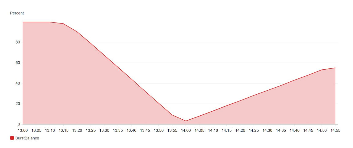
Below CloudWatch diagram shows that I/O credits went down after we did the above experiment. It is very close to 0 percent because we burst 1712 second with around 3000 IOPS.You can also notice that refill started as soon as the above command execution is complete.

How to compute burstbalance and burstduration using AWS CLI commands?

AWS CLI does not have an API to get the value of Burst Duration directly now. But, we can use AWS CLI to get the value of the CloudWatch metric BurstBalance then use it to count the value of Burst Duration for a specific period. The metric BurstBalance provides information about the percentage of I/O credits (for gp2) or throughput credits (for st1 and sc1) remaining in the burst bucket. At the beginning, we create a metric.json file and the content is listed below.

[
{
"Id":"burst_duration",
"Expression":"credit*5400000/100/(3000-500*3)",
"Label":"Credits"
},
{
"Id":"credit",
"MetricStat":{
"Metric":{
"Namespace":"AWS/EBS",
"MetricName":"BurstBalance",
"Dimensions":[
{
"Name":"VolumeId",
"Value":"vol-03d6a25179c93b1a1"
}
]
},
"Period":300,
"Stat":"Minimum",
"Unit":"None"
},
"ReturnData":FALSE
}
]

Then, we execute the command below to get the result.

aws cloudwatch get-metric-data –metric-data-queries file://./metric.json –start-time 2019-08-07T06:00:00Z –end-time 2019-08-07T06:05:00Z

the result is listed below.

{
"MetricDataResults": [
{
"Id": "burst_duration",
"Label": "Credits",
"Timestamps": [
"2019-08-07T06:00:00Z"
],
"Values": [
3600.0
],
"StatusCode": "Complete"
}
]
}

The result shows 3600.0 which means 3600 seconds for the sample time period 2019-08-07T06:00:00Z. The size of our volume vol-03d6a25179c93b1a1 is 500GB. The formula of Burst Duration is (credit balance) / (Burst IOPS – 3*Volume Size). Therefore, the Expression is credit*5400000/100/(3000-500*3) in our metric.json file. credit in the Expression is the percent of remaining IOPS creadits, so credit*5400000/100 equals to your remaining I/O credits. We assume that you would like to burst at 3000 IOPS and the size of our volume is 500GB, so we divide credit*5400000/100 by (3000-500*3). The result show 3600 is correct, because we did not use any I/O credit after we launched the instance. Since we did not use the I/O credit, the value of BurstBalance is 100 which means 100 percent.

You can also use the command below to get the value of BurstBalance.

aws cloudwatch get-metric-statistics –metric-name BurstBalance –namespace AWS/EBS –dimensions

Name=VolumeId,Value=vol-03d6a25179c93b1a1 –start-time 2019-08-07T06:00:00Z –end-time 2019-08-07T06:05:00Z –period 300 –statistics Minimum –unit None

the result is listed below

{
"Label": "BurstBalance",
"Datapoints": [
{
"Timestamp": "2019-08-07T06:00:00Z",
"Minimum": 100.0,
"Unit": "None"
}
]
}

The sample period is 300 seconds, so the value of the Minimum is the minimum value of BurstBalance during the 300 seconds. Friendly reminders, please make sure AWS CLI configuration setting is correct such as the setting of region, and permission of the account before you use the above CLI api

Share this Post :